
The optical fiber — does.
A single cable turns into thousands of virtual sensors along the entire pipeline.
Geotechnical processes — settlement, mining damage, slope creep, scour — develop over years and remain invisible to point inspections. Fiber-optic strain monitoring reveals pipeline behaviour across tens of kilometres, continuously and in real time.
A threat you cannot see until damage occurs
Local settlement beneath a watercourse, slow slope creep or a subsidence trough above a worked deposit can generate strains from tens to several thousand µε — in extreme cases exceeding the yield strength of steel. Periodic inspections show the condition of the asset only at selected moments and points.
PROBLEM
Distributed in time and space
Deformations build up gradually over many kilometres. Individual measurement points cannot capture where and when an anomaly appears.
RISK
Up to thousands of µε
Subsidence troughs and mass movements generate stresses that in extreme cases exceed the yield strength of the pipeline.
RESPONSE
A continuous view of the whole line
Fiber-optic technologies give the operator information about the entire pipeline — continuously over time, with precise chainage location.
The cable as thousands of virtual sensors
Unlike point sensors, the optical fiber is a measuring element distributed continuously along the entire length of the asset. A single cable becomes the equivalent of thousands of virtual sensors every few tens of centimetres. The way it is installed determines what we actually measure:
Strain-coupled
A strain-coupled cable — rigidly attached or grouted to the pipe/ground. It faithfully reproduces the mechanical strain of the structure.
Loose-tube
A loose-tube cable — mechanically decoupled. It measures temperature and is used to compensate for its influence on the strain measurement.
Parallel configuration
Two or more lines (top/bottom, left/right of the pipe) make it possible to determine the curvature and bending direction of the pipeline.
The advantages are a direct consequence of the fiber’s physics: full immunity to electromagnetic interference, no power supply along the route, intrinsic safety (Ex zones), corrosion resistance and multi-year durability. A single cable simultaneously measures strain, temperature and — in acoustic variants — vibration and third-party interference.
How ground movement turns into a signal
Drag the slider to trigger a settlement zone beneath the pipeline. Watch the pipe sag, the fiber stretch, and a characteristic anomaly grow on the continuous ε(z) profile — and see when it crosses the warning and alarm thresholds.
Settlement simulator & strain profile ε(z)
DISTRIBUTED STRAIN SENSING
The thresholds (1000 µε warning / 1500 µε alarm) are illustrative — in practice they are set according to the pipe class, design stresses and acceptance criteria.
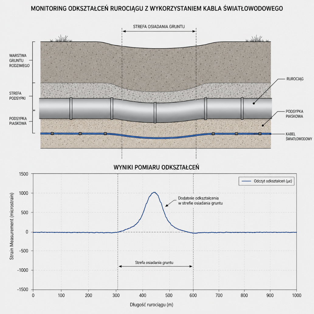
How the optical fiber „senses” strain
The raw measurement is a change in frequency or wavelength of the scattered light. The three techniques differ in physics, range and resolution — and in practice they complement one another within a single system.
① BOTDR — Brillouin scattering
LONG TRUNK LINES · >80 km
A laser pulse interacts with the natural acoustic vibrations (phonons) of the glass, producing Brillouin scattering. The Brillouin shift νB (~10.8–11 GHz at 1550 nm) changes almost linearly: ~0.05 MHz/µε and ~1 MHz/°C. By analysing the signal as a function of the round-trip time (the OTDR principle), we obtain a continuous ε(z) profile.
| Range | up to approx. 25 km (BOTDR), >80 km (BOTDA) |
| Spatial resolution | 0.2–2 m |
| Strain accuracy | approx. ±2 µε |
| Temperature accuracy | approx. ±0.1 °C |
| Main application | long trunk sections, monitoring of entire lines |
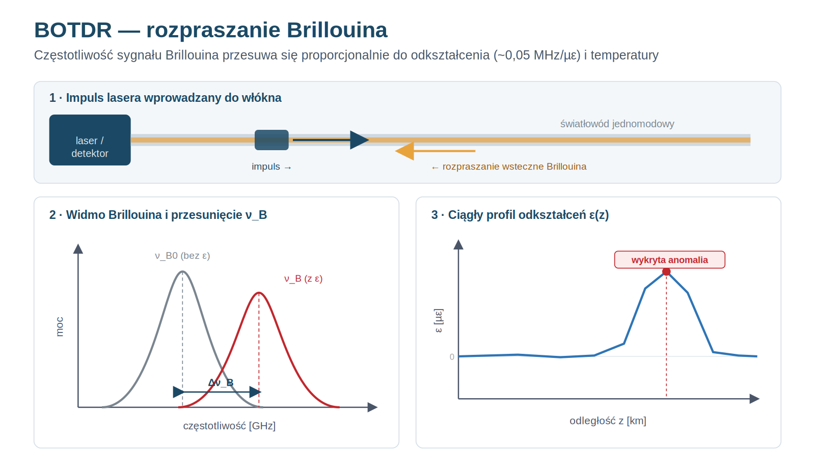
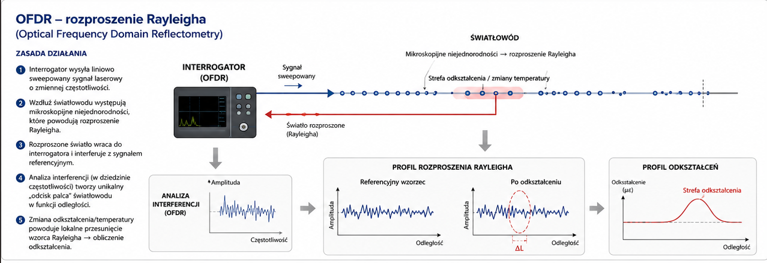
② OFDR — Rayleigh scattering
mm RESOLUTION · 100 m
Every fiber has a unique scattering pattern — an optical „fingerprint”. Under strain, the spectrum of a segment shifts relative to the reference state (baseline). OFDR (a tunable laser + interferometry) uses cross-correlation to convert these shifts into an ε(z) distribution with millimetre resolution.
| Range | up to approx. 100 m |
| Spatial resolution | 0.65 mm |
| Accuracy / sensitivity | ±1 µε, sensitivity ~0.1 µε |
| Temperature accuracy | approx. ±0.1 °C |
| Main application | short critical sections, welds, detailed investigations |
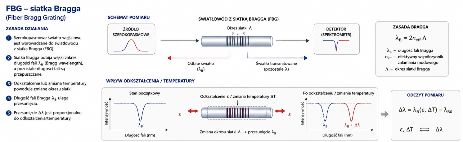
③ FBG — Fiber Bragg Gratings
POINT-BASED · DYNAMICS up to 5 kHz
A Fiber Bragg Grating is a periodic structure (period Λ) in the fiber core. It reflects a narrow band at wavelength λB = 2·neff·Λ. Strain/temperature changes the grating geometry → shifts λB. Sensitivity is ~1.2 pm/µε and ~10–13 pm/°C. Several dozen gratings can be multiplexed on a single fiber; fast interrogation (up to kHz) enables dynamic measurements.
| Measurement type | point-based (discrete sensors at selected locations) |
| Strain sensitivity | approx. 1.2 pm/µε (at 1550 nm) |
| Temperature sensitivity | approx. 10–13 pm/°C |
| Multiplexing | several dozen gratings per fiber |
| Main application | critical points, supports, dynamic measurements |
Interpretation: location, trend, alarm thresholds
The value of the system lies not in a single measurement but in comparing successive campaigns against the baseline and tracking changes over time. Three pillars of interpretation:
Location
Every anomaly is assigned to a chainage along the route — the field inspection is directed precisely to the section at risk.
Trend
The growth of ε between campaigns says more than an instantaneous value — it distinguishes an active process from a stabilised state.
Alarm thresholds
Warning and alarm thresholds automate the response: from notifying the duty officer to dispatching a crew to the field.
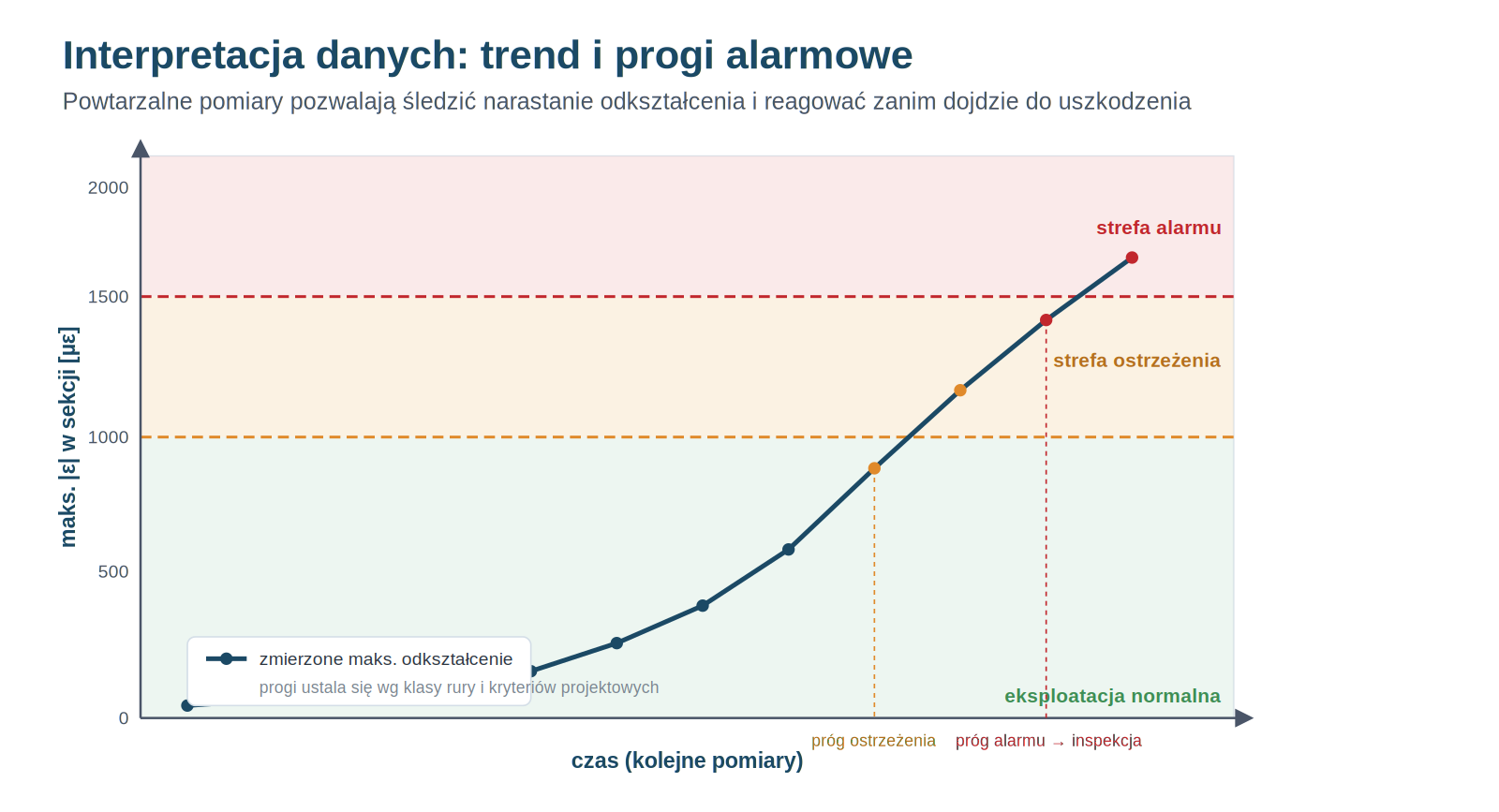
Tracking the strain trend within a section
WARNING / ALARM THRESHOLDS
Successive measurements build up, crossing the warning (1000 µε) and alarm (1500 µε) thresholds — the operator responds before ε reaches critical values.
Typical application scenarios
Anywhere strains develop in a distributed way that is hard to capture with point methods.
Mining damage
Subsidence troughs above areas of mining activity.
Landslides and mass movements
Mountain and slope sections exposed to ground creep.
Crossings under watercourses
River, road and rail crossings — risk of scour and settlement.
Floodplains and permafrost
Freeze/thaw cycles and flooding that cause ground movement.
Construction and pressure tests
Monitoring ε during laying, backfilling and strength testing.
Leaks and third-party interference
Temperature (DTS) and acoustic (DAS) variants detect thermal anomalies and earthworks.
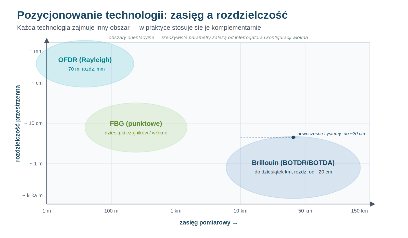
Three techniques, one hybrid system
Brillouin covers tens of kilometres, Rayleigh delivers millimetre resolution, FBG — highly accurate point measurements and dynamics. In real deployments they are combined: the trunk line covered by Brillouin, critical nodes fitted with FBG, welds in OFDR.
| Criterion | Brillouin (BOTDR/BOTDA) | Rayleigh (OFDR) | FBG |
|---|---|---|---|
| Type | distributed | distributed | point-based (multiplexed) |
| Range | 80 km | 100 m | dozens of sensors / fiber |
| Resolution | 20 cm | 0.65 mm | discrete (at a point) |
| ε accuracy | ±2 µε | ~±1 µε | ~±1 µε |
| Dynamic measurement | No | Limited (up to 250 Hz) | yes (up to 5 kHz) |
| Best for | long trunk lines | short critical sections | critical points and dynamics |
Table 1. A summary of the key features of the three fiber-optic strain measurement technologies.
We’ll help you choose the right technology
Every asset is different, and the optimal monitoring system is the result of several technical and operational factors. We’ll share our experience and advise on selecting the technology and configuring a solution tailored to your infrastructure.
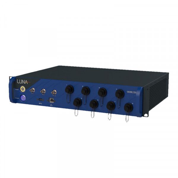 Fiber-optic interrogators and sensors
BOTDR/BOTDA, OFDR (Rayleigh), FBG — selection, installation, baseline and data interpretation within Asset Integrity Management.See all monitoring systems →